Marker Matching

Simple example

To quantify geometric distortion using markers, we need three things:

Ground truth marker location. (We recommend CT imaging for this, but technically you can use the CAD design files)
Distorted marker location
Knowledge of which distorted marker location corresponds to which ground truth marker location

The previous tutorial demonstrated the various ways that MarkerVolumes can be created. In this section, we will demonstrate how these volumes can be automatically matched.

Create a new python file called ‘marker_matching.py’ and copy the below contents into it:

from pathlib import Path
from mri_distortion_toolkit.MarkerAnalysis import MarkerVolume
from mri_distortion_toolkit.MarkerAnalysis import MatchedMarkerVolumes

'''
download example data and unzip:
https://cloudstor.aarnet.edu.au/plus/s/Wm9vndV47u941JU
'''
data_loc = Path(r'C:\Users\Brendan\Downloads\MRI_distortion_QA_sample_data(1)\MRI_distortion_QA_sample_data')
# ^^ update to where you put the sample data!!

# distorted centroids
distorted_volume = MarkerVolume(data_loc / 'MR' / '04 gre_trans_AP_330' / 'slicer_centroids.mrk.json', verbose=False)
distorted_volume_rev = MarkerVolume(data_loc / 'MR' / '05 gre_trans_PA_330' / 'slicer_centroids.mrk.json', verbose=False)

# ground truth centroids
ground_truth_volume = MarkerVolume(data_loc / 'CT' / 'slicer_centroids.mrk.json', verbose=False)

# matched volumes
matched_volume = MatchedMarkerVolumes(ground_truth_volume, distorted_volume,                  ReferenceMarkers=11)
matched_volume.MatchedCentroids.to_csv('_example_data/Matched_Markers.csv')  # for use in later examples

# plot the match
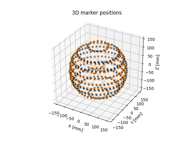
matched_volume.plot_3D_markers()

succesful matching of ground truth to distorted markers

note that we read the marker positions here from previously defined marker files. This is only for speed; high resolution volumes such as CT take a few minutes to process. However, we also provide an example of creating the MarkerVolumes directly from dicom below.

Next steps

The next steps depend on what you are trying to achieve:

If all you want to do is have a way to characterize distortion, the MatchedMarkerVolumes object essentially contains all the information you need, and you can move on to the Reports modules
If you want to calculate the fields and then characterize these fields in terms of spherical harmonics, your next step is field calculation
You can also read on in this section for some more detailed examples of using MatchedMarkerVolumes, or you can come back to this later

An example of things not working well!

In the above example, note the use of the parmeter ReferenceMarkers=11 in MatchedMarkerVolumes. This parameter tells the code to use the 11 inner-most markers in each volume to perform a rigid alignment prior to any attempt to match the markers. This is necessary in this case, because we messed up when we took the CT volume and it is offset in the y-direction! Check for yourself: ground_truth_volume.plot_3D_markers()). Also, we know from when we built this phantom that we placed 11 markers at the center of the phantom for exactly this purpose.

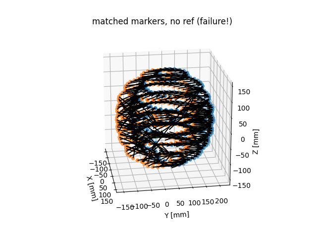
This accidental offset between MR and CT data provides a useful way to demonstrate the limitations of this marker matching approach; we can simply turn this alignment step off and plot the match again:

# matched volumes
matched_volume_no_ref = MatchedMarkerVolumes(ground_truth_volume, distorted_volume)

# plot the match
matched_volume_no_ref.plot_3D_markers()

Not so good!! But a useful example for you of how things might look when the matching process fails. Note that when the code detects such cases, it will prompt you before continuing

What should I do when the matching process fails?

Firstly, you can look over the code docs to see what options are available.

But in general; this can be a hard problem to solve and in cases of extreme situation, I guess our algorithm will fail. So the short answer is log an issue and then start working on a pull request ;-)

Incorporating reverse gradient data

There are two ‘system based’ sources of distortion in MRI: the gradient coils, and B0 inhomogeneity (there are also patient specific effects, which we ignore here.)

Gradient distortion appears in every direction, and is essentially independent of imaging sequence.
For standard sequences, B0 distortion appears only in the readout (frequency encode) direction, and is highly sequence dependent .

These two effects can be seperated out using what is called ‘the reverse gradient technique’; for further explaition see here and here. Instructions for taking such images on a siemens scanner are provided here; this document is about how to analyse such images with this software.

In addition to the volumes you created above, we need to create a ‘reverse gradient’ volume, then we can send them MatchedMarkerVolumes as follows:

# distorted centroids, reversed gradient
distorted_volume_rev = MarkerVolume(data_loc / 'MR' / '05 gre_trans_PA_330' / 'slicer_centroids.mrk.json', verbose=False)

# matched volumes including reversed gradient data
matched_volume_with_rev_data = MatchedMarkerVolumes(ground_truth_volume, distorted_volume,
                                                    ReverseGradientData=distorted_volume_rev, ReferenceMarkers=11)

There is no visible difference, but if you compare matched_volume_with_rev_data.MatchedCentroids with matched_volume.MatchedCentroids You will see that the former has fields for both {x,y,z}gnl and {x,y,z}B0, while the latter only has gnl. This is because when a reverse gradient volume is include, it allows us to seperate the B0 distortion effects from the gradient distortion effects.

How to intepret the reverse gradient data

In the above example, we have two MR images in which the phase encoding gradient (and by extension, frequency encoding gradient) was reversed from PA to AP. We would expect that B0 effects would be prominent in the frequency encode direction and slice encode direction. To check what these are, you can take a look at one of the MR volumes created from dicom_data:

distorted_volume = MarkerVolume(data_loc / 'MR' / '04 gre_trans_AP_330', verbose=False)
for key, value in distorted_volume.dicom_data.items():
    print(f'{key}: {value}')

:warning: warning! dicom_data is only present in MarkerVolumes created from MR dicom images. This is why we recreated the distorted_volume here. You can save the dicom data from such a volume using save_dicom_data()

this will tell you that the frequency encode direction is x, phase encode is y, and slice encode is z. Therefore, from this data we can obtain:

A good measurement of the X gradient disortion
A good measurement of the Z gradient distortion
A good measurement of the effects of B0 distortoin for this sequences
But we do not get a good estimate of the Z gradient distortion, because these markers contain effects from both gradient non-linearity in B0 inhomogeneity that we are unable to seperate

To get a good estimate of the of the Z gradient alone, we would need to take images with the frequency encoding direction in Z. Ideally, we would take three sets of images.

For each reverse gradient pair of images, we should obtain an estimate of B0 distortion. A good sanity check is how consistent these estimates are!

Creating the MarkerVolumes from dicom versus json

Note that in the above code, we read the markers in from a previously exported json files. This is only for speed; you can just as easily create them all directly from dicom, as demonstrated in the marker extraction example

# code to create MarkerVolume from CT; one extra parameter is required:
ground_truth_volume = MarkerVolume(data_loc / 'CT', r_max=300)

We are using the r_max=300 parameter to discount some of the outlier markers that show up. These outliers don’t particularly matter anyway since they are never matched to a distorted marker, but things are tidier if we just get rid of them. A full list of the options for this class is here

Whenever you have a MarkerVolume you can always used the export_to_slicer() method to save the marker positions as json.