Geometry Optimisation Example

The starting point for an optimisation is a working topas model. In this example we are going to optimise the geometry of a simple x-ray collimator. We are going to randomise the values shown in read, and see if we can recover the correct values using the Bayesian optimisation. To guide the optimisation, we will create an objective function which simply measures the difference between the original depth dose curves and profile data and those created by a given set of parameters.

If you are an experienced python and topas user, you should allow 1-2 hours to set up this example (this will get much quicker once you get the hang of it; it takes me about 15 minutes).

Actually running this example will take ~4 hours on a decent computer.

Environmental set up and installation

If you need help getting your environment or with installation set up see here.

Base model and problem overview

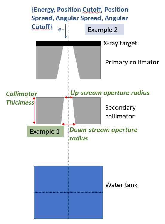
In this example, we will optimise the geometry of an X-ray collimator. The geometry is shown below, with the parameters targeted for optimisation shown in red. The original values for each of these parameters are: Collimator Thickness = 54 mm, Up-stream aperture radius = 1.82 mm, and Down-stream aperture radius = 2.5 mm. This is modelled in two stages: in stage one an electron beam hits the target and the resultant collimated X-ray beam is scored below the secondary collimator. In stage 2, this phase space is used to simulate the dose in the water tank.

In this example, each of these parameters will first be assigned a random value. We will then attempt to recover the original values by constructing a simple objective function based on the differences between the original data and the current iteration.

directory set up

To start with, create a folder somewhere called for instance ‘ApertureOptExample’ (or whatever you want). This is where you will store all the code necessary to run the optimisation. The rest of the instructions assume you are in this working directory.

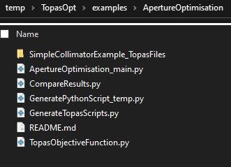
When you have finished working through this example you should have a working directory which looks like this:

Copy the base topas files

The code will need to know where your base model is stored. The base model for this application is available here. Download and unzip this folder, and place the contents inside your working directory (ApertureOptExample in this example). Note that in principle these files can reside anywhere; we are only using the working directory to make this example as simple as possible!

hint: if you are running this example inside a command window use the following commands:

wget -O start_files.zip "https://zenodo.org/records/10369317/files/SimpleCollimatorExample_TopasFiles(2).zip?download=1"
# ^this is all one line!
unzip start_files.zip
rm start_files.zip

Creating GenerateTopasScript.py

The first thing we will be needing is a function that generates your topas script.

Create a python file called ‘temp_GenerateTopasScript.py’ (or whatever you want, the name isn’t important). Copy the below code into it (or use an interactive console if you prefer):

from TopasOpt.TopasScriptGenerator import generate_topas_script_generator
from pathlib import Path

this_directory = Path(__file__).parent  # figures out where your working directory is located

# nb: the order is important to make sure that a phase space files are correctly classified - they should be entered in the same order they will be run
generate_topas_script_generator(this_directory, ['SimpleCollimatorExample_TopasFiles/SimpleCollimator.tps',
 'SimpleCollimatorExample_TopasFiles/WaterTank.tps'])

Tip: CreateTopasScript is a code that takes a code and generates a code that generates a code. If that makes your head hurt you are not alone!

If it worked, you will now have a python function in your Optimisation Directory called GenerateTopasScripts.py.

If you open this script up, you will see that all it has done it copied the contents of the topas file you input into a list, which it returns. At the moment, it’s not very useful because every time it’s called it will copy out exactly the same script! We will change that a bit later; but first it’s a good idea to test this script and see if it actually works.

To test it, run it directly. This will create two scripts in your working directory called SimpleCollimator.tps and WaterTank.tps. They should be almost identical to the input scripts. A few changes are made so we can easily keep track of different optimisation iterations in the phase space files etc.

You can delete temp_GenerateTopasScript.py now if you want to, it has done its job.

warning: There are probably situations which GenerateTopasScripts does not handle well. For instance, CAD file imports are currently unsupported. In general, you should think of the script created at this point as a first draft. You may have to do some further work on it to get it to do exactly what you want. We will make some edits to GenerateTopasScripts.py a bit later on in this example.

Creating RunOptimisation.py

Create a new file called RunOptimisation_main.py (or whatever you want, the name isn’t important). Copy the below code into it:

import numpy as np
from pathlib import Path
from TopasOpt import Optimisers as to

BaseDirectory =  '/home/brendan/Documents/temp'
SimulationName = 'NMtest'
OptimisationDirectory = Path(__file__).parent


# set up optimisation params:
optimisation_params = {}
optimisation_params['ParameterNames'] = ['UpStreamApertureRadius','DownStreamApertureRadius', 'CollimatorThickness']
optimisation_params['UpperBounds'] = np.array([3, 3, 40])
optimisation_params['LowerBounds'] = np.array([1, 1, 10])
# generate a random starting point between our bounds (it doesn't have to be random, this is just for demonstration purposes)
# random_start_point = np.random.default_rng().uniform(optimisation_params['LowerBounds'], optimisation_params['UpperBounds'])
# optimisation_params['start_point'] = random_start_point
optimisation_params['start_point'] = np.array([2.46, 1.62, 35])
# Remember true values are  [1.82, 2.5, 27]
optimisation_params['Nitterations'] = 40
# optimisation_params['Suggestions'] # you can suggest points to test if you want - we won't here.
ReadMeText = 'This is a public service announcement, this is only a test'


Optimiser = to.BayesianOptimiser(optimisation_params=optimisation_params, BaseDirectory=BaseDirectory,
                                 SimulationName='GeometryOptimisationTest_Bayes', 
                                 OptimisationDirectory=OptimisationDirectory, TopasLocation='~/topas37', 
                                 ReadMeText=ReadMeText, Overwrite=True, bayes_length_scales=0.1)
Optimiser.RunOptimisation()

A full list of Optimiser options are here but the inputs we are using this case are described below:

• optimisation_params is the dictionary of parameters we set up in this script, which describe the parameter names, starting values, and allowed bounds.

• BaseDirectory is where you want to store all your optimisations

• SimulationName this particular simulation will be stored

• OptimisationDirectory Is the directory where this script is located. Note that we automate this so there is no need for to hard code it.

• ReadMeText is an optional parameter where you can simply enter some text describing what the optimisation is supposed to be doing. this can be pretty useful when you come back to some case months later!

• Overwrite=True means that the optimiser will empty any files in BaseDirectory / SimulationName. If this option is False, the code will ask you first.

• TopasLocation is the path to your topas installation. If you followed the installation instructions, this will be at ~/topas, which is where the code will look by default.

• KeepAllResults if False, only the last results files are kept (the logs record all results in either case)

Editing GenerateTopasScript.py

Remember from earlier that GenerateTopasScripts.py currently regenerates the original topas scripts. For an optimisation, we need to be able to receive parameters from the optimiser, and build a model reflecting these parameters. Therefore we will have to make some changes to this script!

Whenever GenerateTopasScript is called from the optimiser, it will be passed a dictionary that contains the variables defined in optimisation_params and their current values. We need to edit GenerateTopasScript so that when these parameters change, the topas parameters change accordingly. Firstly, we need to change three lines:

# 1. change
SimpleCollimator.append('d:Ge/SecondaryCollimator/RMin2      = 1.82 mm')
# to
SimpleCollimator.append('d:Ge/SecondaryCollimator/RMin2      = ' + str(variable_dict['UpStreamApertureRadius']) + ' mm')

# 2. change
SimpleCollimator.append('d:Ge/SecondaryCollimator/RMin1      = 2.5 mm')
# to
SimpleCollimator.append('d:Ge/SecondaryCollimator/RMin1      = ' + str(variable_dict['DownStreamApertureRadius']) + ' mm')

# 3. change
SimpleCollimator.append('d:Ge/SecondaryCollimator/HL         = 27 mm')
# to
SimpleCollimator.append('d:Ge/SecondaryCollimator/HL      = ' + str(variable_dict['CollimatorThickness']) + ' mm')

Notice that we have used the same variable names that we set up RunOptimisation.py. These can be called anything you want, they just have to be used consistently.

We will make a few more changes. The original files used 500000 primary particles which are split 1000 times in the target. The resultant phase space is scored just below the collimator, and recycled 200 times in the water tank simulation. This took around 1 hour to run on 16 multi threaded cores.

We don’t actually need especially high quality data to guide the optimser, so I’m going to reduce the number of primary particles by a factor of 10:

# change
SimpleCollimator.append('ic:So/Beam/NumberOfHistoriesInRun = 500000')
# to
SimpleCollimator.append('ic:So/Beam/NumberOfHistoriesInRun = 50000')

Hint In many cases, it is desirable to simple check that the optimisation will run through a complete iteration before running anything computationally intensive. To test that, you could just change NumberOfHistoriesInRun to e.g. 100

Hint: Figuring out the optimal trade-off between simulation time and simulation noise is something that can take quite a while to get right! It can be helpful to run the same simulation e.g. 10 times, and assess the variance in the objective function against the accuracy of the result you hope to obtain with the optimization. You can do such experiments quite easily using GenerateTopasScripts.py

Creating TopasObjectiveFunction.py

Finally, create a file called TopasObjectiveFunction.py. The name of this does matter!

The only things this file must do is

1. Contain a function called TopasObjectiveFunction which:

   1. Receive two inptuts from the optimiser: the location of the results, and the current iteration

   2. Return a value for the objective function to the optimiser.

A very simple example of a function which meets these requirements is below:

import numpy as np

def TopasObjectiveFunction(ResultsLocation, iteration):
    return np.random.randn()

Of course, this is pretty useless as an objective function since it returns a random number that has nothing to do with the results! But it illustrates a very useful principle: all this function has to do is take two parameters and return a number. You can do whatever you want in between.

A more sensible objective function must do a few more things:

• Read in the latest results,

• Extract some metrics from them

• Calculate an objective value based on those results.

The actual objective function we will use in this example fulfills these criteria, and is copied below. Copy this code into TopasObjectiveFunction.py and update the location of GroundTruthDataPath to wherever you downloaded the input topas scripts.

import os
from TopasOpt.utilities import WaterTankData
import numpy as np
from pathlib import Path

def CalculateObjectiveFunction(TopasResults, GroundTruthResults):
    """
    In this example, for metrics I am going to calculate the RMS error between the desired and actual
    profile and PDD. I will use normalised values to account for the fact that there may be different numbers of
    particles used between the different simulations
    """

    # define the points we want to collect our profile at:
    Xpts = np.linspace(GroundTruthResults.x.min(), GroundTruthResults.x.max(), 100)  # profile over entire X range
    Ypts = np.zeros(Xpts.shape)
    Zpts = GroundTruthResults.PhantomSizeZ * np.ones(Xpts.shape)  # at the middle of the water tank

    OriginalProfile = GroundTruthResults.ExtractDataFromDoseCube(Xpts, Ypts, Zpts)
    OriginalProfileNorm = OriginalProfile * 100 / OriginalProfile.max()
    CurrentProfile = TopasResults.ExtractDataFromDoseCube(Xpts, Ypts, Zpts)
    CurrentProfileNorm = CurrentProfile * 100 / CurrentProfile.max()
    ProfileDifference = OriginalProfileNorm - CurrentProfileNorm

    # define the points we want to collect our DD at:
    Zpts = GroundTruthResults.z
    Xpts = np.zeros(Zpts.shape)
    Ypts = np.zeros(Zpts.shape)

    OriginalDepthDose = GroundTruthResults.ExtractDataFromDoseCube(Xpts, Ypts, Zpts)
    CurrentDepthDose = TopasResults.ExtractDataFromDoseCube(Xpts, Ypts, Zpts)
    OriginalDepthDoseNorm = OriginalDepthDose * 100 /np.max(OriginalDepthDose)
    CurrentDepthDoseNorm = CurrentDepthDose * 100 / np.max(CurrentDepthDose)
    DepthDoseDifference = OriginalDepthDoseNorm - CurrentDepthDoseNorm

    ObjectiveFunction = np.mean(abs(ProfileDifference)) + np.mean(abs(DepthDoseDifference))
    return ObjectiveFunction


def TopasObjectiveFunction(ResultsLocation, iteration):

    ResultsFile = ResultsLocation / f'WaterTank_itt_{iteration}.bin'
    path, file = os.path.split(ResultsFile)
    CurrentResults = WaterTankData(path, file)
    
    GroundTruthDataPath = str(Path(__file__).parent / 'SimpleCollimatorExample_TopasFiles' / 'Results')
    # this assumes that you stored the base files in the same directory as this file, updated if needed
    GroundTruthDataFile = 'WaterTank.bin'
    GroundTruthResults = WaterTankData(GroundTruthDataPath, GroundTruthDataFile)
    
    OF = CalculateObjectiveFunction(CurrentResults, GroundTruthResults)
    return OF

This code can serve as a useful template for for developing your own objective functions, but as mentioned: your objective function can do anything you want, as long as it take the two parameters ResultsLocation and iteration and return a number.

The objective function we are using is simply the sum of the absolute differences between a profile at iso center and a depth dose curve. Note that both the current and original data are normalised to account for the fact that different numbers of primary particles are being used.

Hint: if you want a guaranteed way to impress your friends and family, you can tell them that this is an L1 norm objective function

Running the example

You now have all the building blocks in place to run this example. To do so, you simply need to run RunOptimisation_main.py:

# from a command window:
python RunOptimisation_main.py 

Note that although I have tried to make a relatively light weight example here, it still requires a substantial server to run on. I ran this example on a server with 16 multi-threaded CPUs and it took around 5 minutes per iteration. To complete 40 iterations therefore will take ~ 4 hours.

warning: I have used very aggressive variance reduction in this example. Always be careful with implementing variance reduction techniques.

Interpreting the results

Ok, you’ve gone away and drunk several beers while the optimisation was running, and you are now ready to see how it did!

Navigate to whatever you set up as BaseDirectory / SimulationName in your RunOptimisation script. An explanation of the folders you see here:

• logs: Contains log files from the optimisers and results from the optimisation.

  • TopasLogs: contains the output from each topas simulation that was run. If your topas sims ever crash, this is a good starting point to figure out why

  • SingleParameterPlots: This contains the estimate of how the objective function will change as a function of each parameter, assuming all other parameters are held at the (current) optimal value,

• Results: Contains the topas simulation outputs. By default it will contain the result of every simulation you ran. In some cases this will be a lot of unnecessary data, and you can set KeepAllResults=False

• TopasScripts: Contains the scripts used to run each iteration.

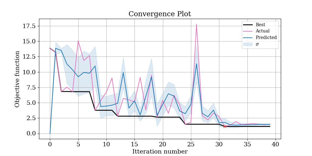
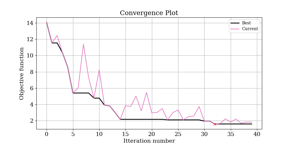
To start with, have a look at logs/ConvergencePlot.png, This will show you the actual and predicted value of the objective function at each iteration. Ideally, you should see that the predictions get better (better correlation) with more iterations. The best point found is marked with a red cross.

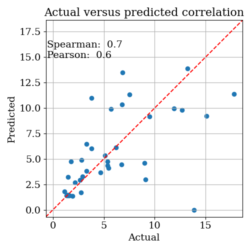
Next, open logs/CorrelationPlot.png. This shows a scatter plot of the predicted versus actual objective function across all iterations. If the gaussian process model is working well, you should see reasonable correlation, and both correlation metrics should be > 0.5.

Note: the gaussian process model doesn’t have to be particularly accurate to be useful; it just has to correlate reasonably well with the true objective function

If the correlation isn’t great, you could have a look at logs/RetrospectiveModelFit.png. This plots what the model predicts after it has seen each point. If this also isn’t working, you have a serious problem with the model, since predicting something that has already happened isn’t very difficult!! In this case, if your model didn’t show great correlation, it’s most likey simply due to the low number of iterations we have run.

Take a look at the plots in logs/SingleParameterPlots. These plots show the gaussian process predicted objective function value as a function of each parameter, while the other parameters are held at their optimal value.

warning: these plots show the value of the objective function predicted by the model. In the instances where the correlation between the predicted and actual objective functions is high, you can trust that these plots at least correlate with reality. But if the correlation is low, these plots are essentially nonsense.

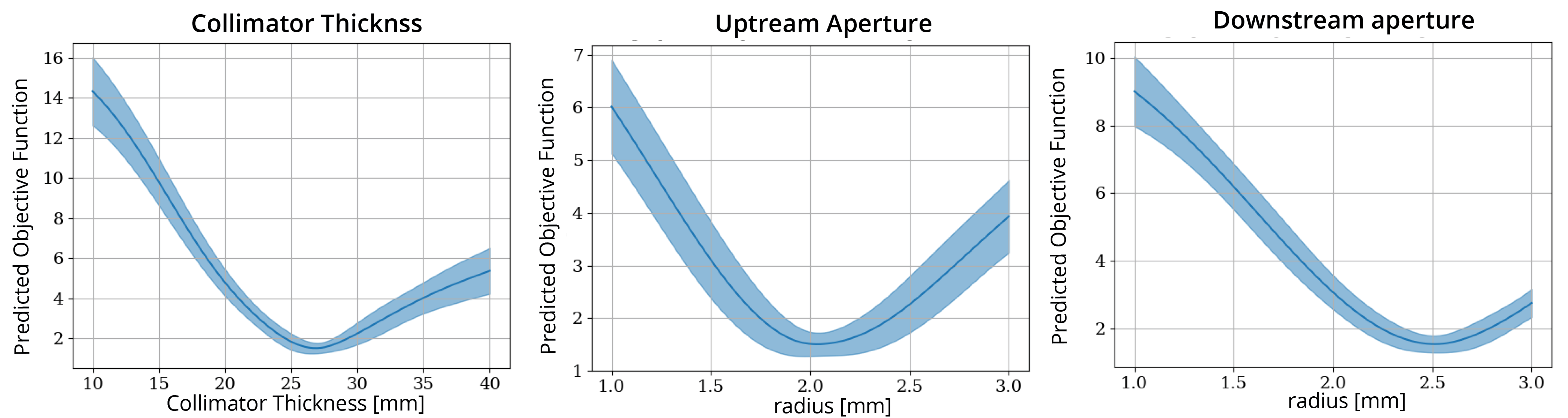In this case, the correlation values are reasonable, so we should be reasonably confident in these plots. This is also indicated by the fact that the models own estimate of uncertainty (indicated by the blue shading) is low.

Finally, open OptimisationLogs.txt and scroll to the bottom. This will tell you what the best guess for each parameter was. After running this example for 40 iterations, I got the following result:

Best parameter set: Itteration: 31., CollimatorThickness:  27.29, UpStreamApertureRadius:  1.95, DownStreamApertureRadius:  2.54, ObjectiveFunction: 1.12

Parameter	Original Value	Random Starting Value	Recovered Value
CollimatorThickness HVL	27 mm	39.9 mm	27.3 mm (1.1% off)
UpStreamApertureRadius	1.8 mm	1.14 mm	2.0 mm (9% off)
DownStreamApertureRadius	2.5 mm	1.73 mm	2.5 mm (0% off)

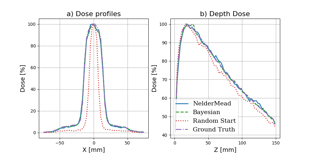
This is pretty good! In just 40 iterations, we recovered the original values to within 10% of their original values. Compare this to a grid search approach: if we split each variable into 10, it would require 1000 iterations, and the spacing between solutions would still be larger than the accuracy obtained here. It is also helpful to interpret these results in the context of the single parameter plots shown above. These plots suggest that the least sensitive parameter is the Upstream Aperture, which is the parameter we have the largest error in (9%). We might therefore expect that the dose profiles are not all that sensitive to this error. A comparison between the starting results and optimized results is shown at the end of this example.

Comparison with Nelder-Mead optimiser

Another optimisation algorithm commonly applied to these types of problems is the NelderMead algorithm. To switch to the NelderMead optimiser, you just have to change one line inside RunOptimisation.main:

# change
Optimiser = to.BayesianOptimiser(optimisation_params, BaseDirectory, SimulationName, 	 OptimisationDirectory, TopasLocation='~/topas37', ReadMeText=ReadMeText, Overwrite=True, KeepAllResults=True)

# to
Optimiser = to.NelderMeadOptimiser(optimisation_params=optimisation_params, BaseDirectory=BaseDirectory,
                                   SimulationName='GeometryOptimisationTest_NM', OptimisationDirectory=OptimisationDirectory,
                                   TopasLocation='~/topas37', ReadMeText=ReadMeText, Overwrite=True, KeepAllResults=True,
                                   NM_StartingSimplex=0.2)

# note we changed SimulationName so we won't overwrite the previous results

The convergance plot is shown below:

and the results:

Parameter	Original Value	Random Starting Value	Recovered Value
CollimatorThickness	27 mm	39.9 mm	27.9 (3.3 %)
UpStreamApertureRadius	1.82 mm	1.14 mm	2.26 (24.2 %)
DownStreamApertureRadius	2.5 mm	1.73 mm	2.51 (0.4 %)

In this case, the NelderMead Optimiser has also done a great job, almost as good as the Bayesian optimiser. For complex objective functions, the NelderMead approach has a tendency to get stuck in local minima. However for simple situations, it will often converge mode quickly than the Bayesian approach, since it doesn’t have to learn the underlying objective function to be effective.

Comparison with ground truth data

To compare multiple results we have included a function in utilities.compare_multiple_results, which is used like this:

from TopasOpt.utilities import compare_multiple_results

ResultFiles = ['Z:/Documents/temp/NM_OptAperture/Results/WaterTank_itt_39.bin',
              'Z:/Documents/temp/BayesOptAperture/Results/WaterTank_itt_31.bin',
              'Z:/Documents/temp/BayesOptAperture/Results/WaterTank_itt_0.bin',
              'C:/Users/bwhe3635/Documents/temp/TopasOpt/docsrc/_resources/WaterTank.bin']

custom_legend = ['NelderMead','Bayesian','Random Start','Ground Truth']

compare_multiple_results(ResultFiles, custom_legend_names=custom_legend)

Using this code, we can generate the following figure:

Improving these results

There are number of things you could do to improve these results, many of which are explained in a bit more detail in the next steps section:

• Run more iterations

• Nelder-Mead: change the starting point, change the starting simplex

• Making a better objective function: we arbitrarily chose an objective function based on a depth dose curve and profiles, but we could probably find some more sensitive metrics.

• assess the noise in the objective function and decide if we need to run more particles or not. Note that if there is 10% noise, this is a rough limit on how accurate to expect the optimisation to be.